Abstract¶

In image subtraction analysis (also called “difference image analysis”, or DIA), an observation image is subtracted from a template image in order to identify transients from either image. To perform such analysis, the observation must be astrometrically aligned to the template image, and the PSFs of the two images are matched. Arising primarily due to slight astrometric alignment or PSF matching errors between the two images, flux “dipoles” are a common artifact often observed in image differences (and even if these issues were perfectly corrected, unless the two images were obtained at similar zenith distances, differential chromatic refraction [DCR] would still lead to such artifacts). These dipoles will lead to false detections of transients unless correctly identified and eliminated. Moreover, accurate measurement of the flux dipoles can enable evaluation of methods for mitigating the processes which caused them. There is a strong covariance between dipole separation and source flux, such that dipoles arising from faint, but highly-separated sources are nearly indistinguishable from those coming from bright, closely-separated sources. We proposed to alleviate this degeneracy by incorporating data from the two original “pre-subtraction” (i.e., registered and PSF-matched) images to constrain the fit. We describe an implementation of the proposed solution in a new DipoleMeasurementPlugin and Task, and show that it leads to significantly improved solutions, particularly in the low signal-to-noise regime.

Summary of existing LSST stack implementation (ip_diffim, dipoleMeasurement)¶

The current dipole measurement task in the LSST stack is initialized with SourceDetection performed on the image difference, in both positive and negative modes to identify significant pos. and neg. sources. These pos. and neg. source catalogs are merged to identify candidate dipoles with overlapping pos./neg. footprints. The measurement task then performs two separate measurements on these dipole candidates (i.e., those footprints with two sources):

1. A “naive” dipole measurement which computes a 3x3 weighted moment around the nominal centroids of each peak in the Source Footprint. It estimates the pos./neg. fluxes correspondingly as sums of the pos./neg. pixel values within the merged footprint.
2. Measurements resulting from a weighted least-squares joint (dual) PSF model fit to the negative and positive lobes simultaneously. This fit simultaneously solves for the negative and positive lobe centroids and fluxes using non-linear least squares minimization. The existing method is implemented in C++ and uses the minuit2 C++ optimization library with standard parameters (tolerances) for least-\(\chi^2\) minimization of of six parameters: two centroids and two fluxes.

The two measurements are performed independently and do not appear inform each other; in other words the centroids and fluxes from the naive dipole measurement are not used to initialize the starting parameters in the least-squares minimization.

Evaluation of dipole fitting accuracy, robustness¶

We implemented a faux dipole generation routine with a double Gaussian PSF (default \(\sigma_{PSF} = 2.0\) pixels; see notebooks for additional parameters) and realistic non-background-limited (Poisson) noise. We then implemented a separate 2-D dipole fitting function in “pure” python (we used the lmfit package, which is a wrapper around scipy.optimize.leastsq() that allows for parameter constraints and additional useful tools for evaluating model fit accuracy and quality). The dipole (and the function which is minimized) is generated using a Psf as implemented in the LSST stack.

Using similar constraints (i.e., none), the new python optimization results in model fits with similar characteristics to those of the dipoleMeasurement code. For example, a plot of recovered x-coordinate of dipoles of fixed flux with gradually increasing separations is shown in Figure 1:

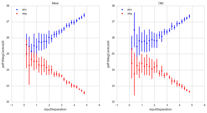
Figure 1 Comparison of recovered dipole centroid x-coordinates for the “New” pure-python dipole fitting routine, and the (“Old”) existing dipoleMeasurement routines, for dipoles of fixed flux with gradually increasing separations. Note that in all figures, including this one, “New” refers to the “pure python” dipole fitting routine, and “Old” refers to the fitting in the existing dipoleMeasurement code. These are for (default) PSFs with \(\sigma_{PSF}=2.0\). All spatial units are pixels.

A primary result of comparisons of both dipole fitting routines showed that if unconstrained, they would have difficulty measuring accurate fluxes (and separations) at separations smaller than \(\sim 1 \sigma_{PSF}\). This is best seen in Figure 2, which shows fitted dipole fluxes as a function of dipole separation for a number of realizations per separation (and input flux of 3000).

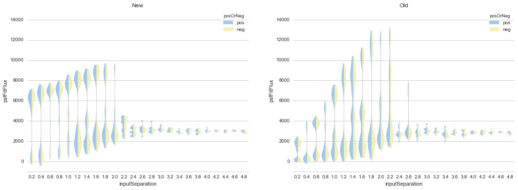
Figure 2 Comparison of recovered dipole fluxes as a function of dipole separation for the “New”, and the “Old” (existing) dipoleMeasurement routines, for dipoles of fixed flux (3000) and gradually increasing separations (pixels). Here, pos -itive and neg -ative lobe flux estimates are shown side-by-side in blue and yellow respectively, on the same (positive) flux axis. Because in all cases the source flux was set at 3000, we expect all measured fluxes to have the same value. This clearly breaks down when the dipole separation falls below the PSF \(\sigma_{PSF}\).

Below we investigate this issue and find that it arises from the high covariance between the dipole separation and source flux, which prevents achieving accurate optimization, especially at low signal-to-noise in the diffim.

Of note, the new python-implemented optimization is \(\sim 2 \times\) faster than the existing C++ dipoleMeasurement implementation. Further investigation and timings of the existing implementation showed that it performed a complete optimization of a single dipole in less than \(\sim 20\) ms, and the new python-implemented version runs in \(\sim 10\) ms on my Macbook Pro, even though it is fitting to \(3 \times\) the data of the original implementation.

Additional comparisons may be found in the IPython notebooks.

Generic dipole fitting complications¶

There is a degeneracy in dipole fitting between closely-separated dipoles from bright sources and widely-separated dipoles from faint sources. This is further explored using 1-d simulated dipoles in this notebook.

An example is shown in figure_3:

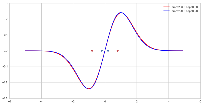
Figure 3 Two example 1-d dipoles exemplifying covariance between dipole flux (here, parameterized by amp) and separation (sep). Although the parameters are significantly different, the dipoles themselves are indistinguishable.

There are many such examples, and this strong covariance between amplitude (or flux) and dipole separation is most easily shown by plotting error contours from a least-squares fit to simulated 1-d dipole data, such as the one in figure_4.

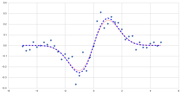
Figure 4 Example simulated data (points) based upon parametric 1-d dipole (blue dashed line) and resulting least-squares fit (red dotted line).

The error contours for this fit are shown in figure_5.

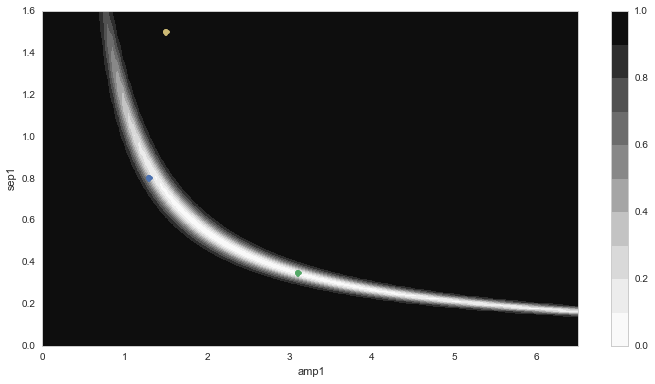
Figure 5 \(\chi^2\) error contours for a dipole fit to the data in figure_4. The blue dot indicates the input parameters (used to generate the data), the yellow dot shows the starting parameters for the minimization and the green dot indicates the least-squares parameters.

Possible solutions and tests¶

This dipole parameter degeneracy is a big problem if we are going to estimate dipole parameters using the subtracted data alone. Three possible solutions are:

1. Use starting parameters and parameter bounds based on measurements from the pre-subtracted images (obs. and template) to constrain the dipole fit.
2. Include the pre-subtracted image data in the fit to constrain the minimization.
3. A combination of (1.) and (2.).

It is noted that these solutions may not help in all cases of dipoles on top of bright backgrounds (or backgrounds with large gradients), such as cases of a faint dipole superimposed on a bright background galaxy. Note that these cases will be rare, but not exceedingly so. One option is to adjust the weighting of the pre-subtracted image data (i.e., in [2] above) to enable the diffim data to dominate, especially in such cases. An alternative that we investigate below is (simultaneously with the dipole fitting, or as a pre-optimization step) to fit parameters for a linear gradient in the pre-subtracted images. This latter option was deemed preferable because it does not require the setting of an (arbitrary) weight parameter.

For example, in figure_6, we show the results (analogous to those in figure_5) of performing a least-squares fit to the same data as in figure_4, but also including the “pre-subtraction” image data as two additional data planes. In this example, the pre-subtracted data points were (arbitrarily) down-weighted to 5% (1/20) relative to the diffim data points for the least-squares fit. The degeneracy is still evident (because of the significant down-weighting of the pre-subtraction data) but even so, the final estimated parameters are very close to the input.

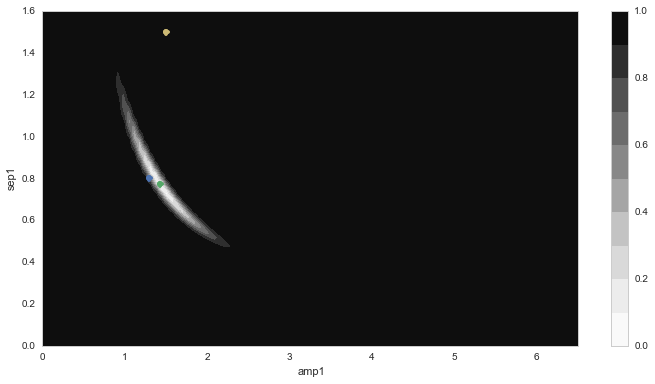
Figure 6 \(\chi^2\) error contours for a dipole fit to the data in figure_4 (see figure_5 for a description). In this case, the pre-subtraction data were included to constrain the fit.

The same degeneracy as described above for 1-d dipoles is also seen in simulated 2-d dipoles, as shown in this notebook. First, a brief overview. In Figure 7 we show a simulated 2-d dipole and the footprints for positive and negative detected sources in the image:

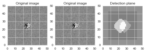
Figure 7 Simulated 2-d dipole and masks showing detected (positive and negative) sources. Input parameters for this example: flux = 3000 ADU; separation = 0.4 pixels.

The least-squares model fit and residuals are shown in figure_8:

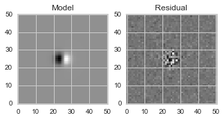
Figure 8 Model fit and residuals for simulated 2-d dipole shown in Figure 7.

A contour plot of \(\chi^2\) error contours (Figure 9) shows a similar degeneracy as that in the 1-d dipoles (figure_6), here between dipole flux and x-coordinate of the positive dipole lobe (top). This is also seen in the covariance between x- and y-coordinate of the positive lobe centroid, which points generally toward the dipole centroid (bottom):

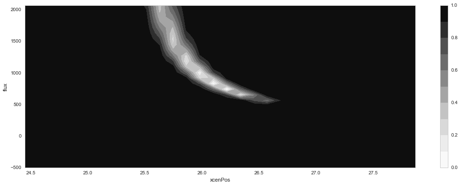
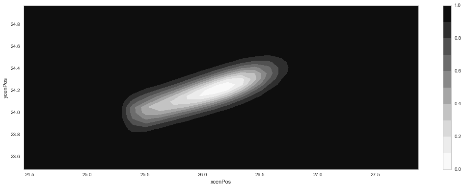
Figure 9 \(\chi^2\) error contours for a 2-d dipole fit to the data in Figure 7, analogous to figure_5. Top: error contours showing covariance between dipole flux and x-coordinate of the positive lobe. Bottom: contours for x- and y- coordinate of the positive lobe.

These contours appear very similar for fits to closely-separated and widely-separated dipoles of (otherwise) similar parameterization (see the notebook for more).

Unsurprisingly, as shown above for the 1-d dipoles, including the original (pre-subtraction) image data for fitting 2-d dipoles serves to significantly constrain the fit and reduce the degeneracy. Increasing the weighting of the pre-subtraction data improves this performance (contours not shown but are available in the IPython notebooks).

Conclusions and Plans¶

Given the analysis of the previous subsection, we have chosen to integrate the pre-subtraction image data in the dipole characterization task for DIA dipoleMeasurement. Two primary cases where this scheme might fail include (1) if the source falls on a bright background or a background with a steep gradient then the pre-subtraction data may provide an inaccurate measure of the original source; and (2) it will require passing the two pre-subtraction image planes (and their variance planes) to the dipole characterization task, and thus a potential slow-down of 3-fold. Issue #1 above may be alleviated in cases of steep background gradients observed in the pre-subtraction footprints by down-weighting the pre-subtraction data relative to the diffim data (as was done in figure_6), in order to decrease the likelihood of an inaccurate fit. This option is still likely to fail in certain cases, and also requires the (arbitrary) selection of a user-definied weight parameter. An alternative solution is to include estimation of parameters to fit the background gradients in the pre-subtracion images. This has the drawback of requiring fitting of additional parameters (three for a linear gradient), while removing the necessity for an additional user-tunable parameter.

Recommendation: Test the dipole fitting including using the additional (pre-subtraction) data planes, including simulating bright and steep-gradient backgrounds. Investigate the tolerance of very low weighting (5 to 10%) or additional parameters to (pre-) fit any background gradients on the pre-subtraction planes to evaluate relative improvement in fit accuracy. Below we show the results for both of these options.

After updating the dipole fit code to include the pre-subtraction images (here again with 5% weighting), as shown in this notebook, the accuracy once again improves.

The new (constrained) result, fitting to the same simulated dipole data, which, notably does not include any gradients in the pre-subtraction images is shown in Figure 10 (note the difference in axis limits):

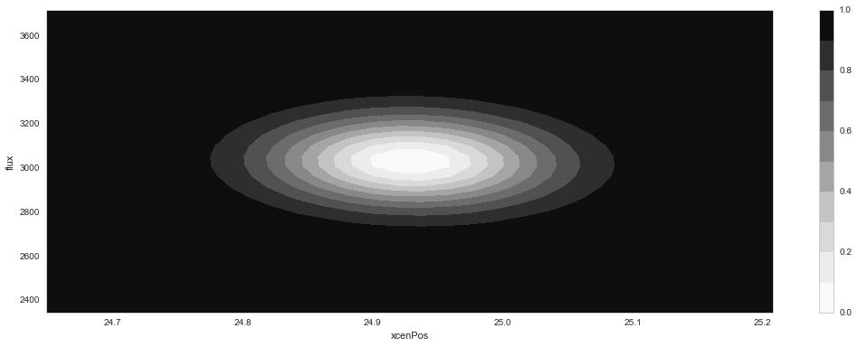
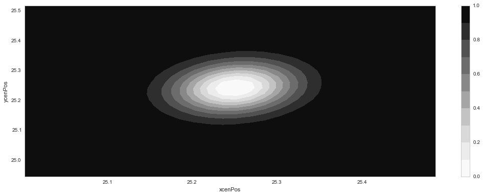
Figure 10 \(\chi^2\) error contours for a 2-d dipole fit to the data in Figure 7, analogous to Figure 9, but in this case integrating the 5%-weighted pre-subtraction image data. Top: error contours showing covariance between dipole flux and x-coordinate of the positive lobe. Bottom: contours for x- and y- coordinate of the positive lobe.

In this case, adding the 5% weighted constraint to the fit unsurprisingly improves the flux measurements for a variety of dipole separations, as shown in Figure 11 (which may be directly compared with Figure 2, generated with no constraint).

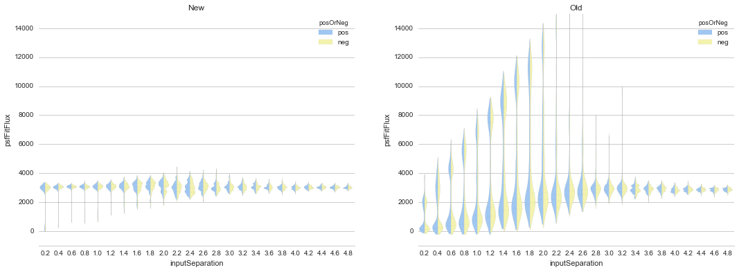
Figure 11 Comparison of recovered dipole fluxes as a function of dipole separation for the “New” constrained method, and the “Old” (existing) dipoleMeasurement routines, for dipoles with fixed flux (3000) and gradually increasing separations (pixels). See Figure 2 for comparison.

Likewise, dipole separations are more accurately measured as well.

Accounting for gradients in pre-subtraction images¶

After adding (identical, linear) background gradients to the pre-subtraction images, fits which down-weighted the pre-subtraction image data but did not include parameters for background estimation in the fits resulted in decreased dipole measurement accuracy (although still significantly improved relative to the original, naive version). This is shown below in Figure 12 (again, see Figure 2 and Figure 11 for comparison). In this case we used fainter sources (1000 vs. 3000 in previous examples) to increase the likelihood of inaccurate results.

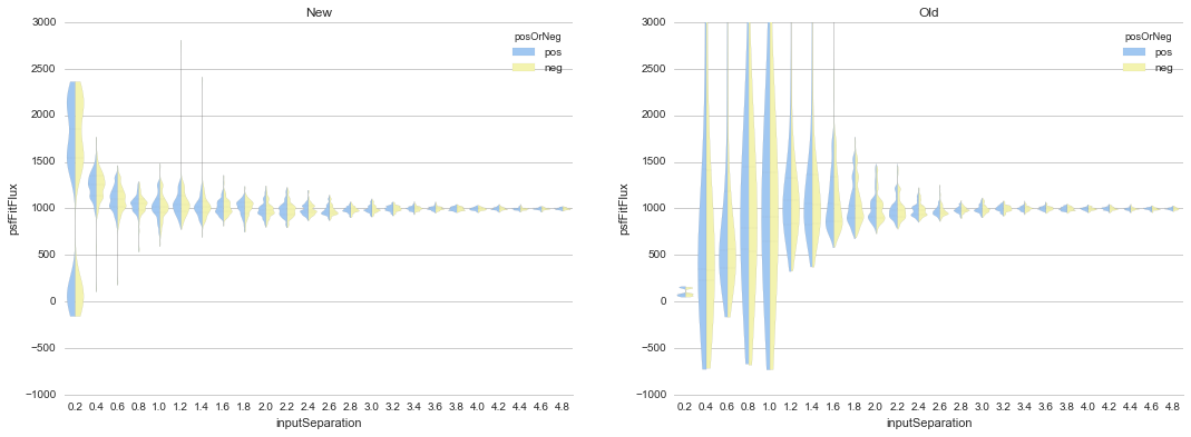
Figure 12 Comparison of recovered dipole fluxes as a function of dipole separation for the “New” constrained method, versus the “Old” (existing) dipoleMeasurement routines, for dipoles on top of background gradients, with fixed flux (1000) and gradually increasing separations (pixels). In this case, we did not include any parameter estimation to measure the background gradients in the pre-subtraction images. See Figure 11 for comparison.

However, once we incorporated estimation of background parameters (in this case, three parameters for a linear background gradient), the fit accuracy returned to its nominal level, as shown below in Figure 13.

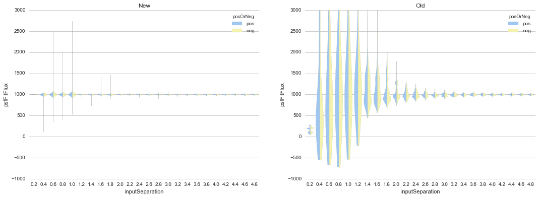
Figure 13 Comparison of recovered dipole fluxes as a function of dipole separation for the “New” constrained method, versus the “Old” (existing) dipoleMeasurement routines, for dipole sources on top of background gradients, and with fixed flux (1000) and gradually increasing separations (pixels). In contrast to Figure 12, here we did include 1st-order polynomial parameters to estimate and remove the background gradients in the pre-subtraction images.

We performed additional evaluations of fit accuracy as a function of gradient steepness, and found that, at least for simple, linear background gradients, no realistic level of gradient steepness could “break” the fitting algorithm that incorporated the background gradient as part of the fit. We did not explore higher-order or nonlinear backgrounds to investigate this claim any further at this time. However, we have implemented the capability of fitting up to a second-order polynomial gradient (i.e, 6 additional parameters) as an option, as we describe below.

DipoleMeasurementTask refactored as DipoleFitTask: implementation details¶

As currently implemented, the new DipoleFitTask is a subclass of SingleFrameMeasurementTask with a new run method which accepts separate posImage and negImage afw.image.Exposure parameters in addition to the default exposure. There is a corresponding DipoleFitPlugin with a measure method that also accepts the additional two exposures as parameters.

The configuration of the new DipoleFitTask is handled by a DipoleFitConfig which contains parameters which affect the least-squares optimization (weights, tolerances and background gradient parameterization), and thresholds for using the fit results to classify the source as an actual dipole.

The algorithm itself utilizes the lmfit python package to perform non-linear least-squares optimization. As mentioned above, lmfit provides a wrapper around the Levenberg-Marquardt implementation provided by scipy.optimize.leastsq(), and additionally allows for parameter constraints and additional useful tools for evaluating model fit accuracy and quality. These latter features will be useful for improving optimization results, as well as for assessing whether an apparent dipole source is truly described by the dipole model.

The dipole model is parameterized by the floating-point pixel centroids of the positive lobes (four parameters) and their fluxes (two additional parameters, unless the constraint is imposed that both lobes’ fluxes are equal). It is constructed using the Psf which has been previously characterized for the diffim. Typically the Psf of the diffim will be identical to those of the two pre-subtraction images which have been PSF-matched in a prior step.

The background gradients in the two pre-subtraction images are presumed to be identical and thus they add either one, three or six additional parameters for a 0th, 1st, or 2nd-order polynomial model (default is 1st). Update(1): The implementation was updated to pre-fit the background gradient to only the pixels outside of the footprint (but within the footprint bounding box) via least-squares (numpy.linalg.lstsq) which is significantly more efficient than including the gradient as part of a joint nonlinear dipole fit. Thus, the gradient is removed (subtracted) from the pre-subtraction image data prior to conducting the dipole parameter estimation. Update(2): The background is now fit to a 2nd-order Chebyshev polynomial using afw.math.makeBackground, which adds flexibility and robustness, in addition to being slightly more efficient than the linear model fitting described above.

Parameter initialization is an important factor affecting robustness of the optimization. The initial centroids are set as the pixel coordinates of the peak (negative and positive) measurements in the footprint. Flux(es) are initialized to the estimated total flux in the background-subtracted pre-subtraction images. The backgrounds are all assumed to be zero for the diffim, as well as for the background gradient-subtracted, pre-subtraction images.

While generally the optimization is robust given the parameter initialization described above, we also impose bounds on their values, which additionally improves the estimation and prevents the optimization from leading to unrealistic values in rare cases. These bounds include constraining the dipole centroids to remain within \(k \times \sigma_{PSF}\) of their initial values (where \(k\) is a tuneable parameter, currently set to 5), and constraining the fluxes to be positive.

Finally, the algorithm passes the above model, parameters, and their initial values and constraints to the lmfit.fit method. It should be noted that lmfit.fit computes the weighted \(\chi^2\) statistic internally, and we simply supply the function that generates the model given the parameters. The resulting parameter estimates and their standard errors, and the model fit \(\chi^2\), \(\chi^{2}_{\nu}\), are extracted and all results are returned by the algorithm. Additional estimates of metaparameters such as dipole orientation and separation, overall centroid, and SNR are computed separately by the DipoleFitPlugin and added to the source record.

Further recommendations, implementation necessities, and future tests¶

1. Evaluate the necessity for separate parameters for pos- and neg- dipole lobes.
2. Utilize the spatially varying Psf, if one exists.
3. Investigate other optimizers, including iminuit possibly more robust and/or more efficient minimization? Update: initial tests suggest that iminuit is actually slightly less efficient than the current lmfit-based optimization due to increased numbers of function calls which is difficult to tune.
4. Only fit dipole parameters using data inside footprint and background parameters outside footprint (but inside footprint bounding box).
5. Correct normalization of least-squares weights based on variance planes. Currently, the variance in the convolved subtracted image is questionable, and the variance in the diffim does not seem to correctly reflect the variance in the pre-subtraction images. Until we get this right, the correctly normalized $chi^2$ estimates will be wrong.

Conclusions¶

We have thoroughly evaluated the task of accurately measuring “dipoles” observed in image differences. Through simulations, we found that the existing task which performed such a measurement using solely the diffim data was inefficient and resulted in inaccurate recovery of correct centroids and fluxes. Including the pre-subtraction image data in the fit serves to constrain these parameters, but only after potential background gradients are subtracted from those data. We have implemented such a procedure for the LSST ip_diffim pipelines which performs these tasks, and thus achieves dipole measurement with significantly greater accuracy at roughly 2x greater runtime efficiency.

Appendix I. IPython notebooks¶

All figures and methods investigated for this report were generated using IPython notebooks. The relevant notebooks may be found in this repo. Much of the code in these notebooks is exploratory; below are the highlights (i.e., the ones from which the figures of this report were extracted):

• Final, versions of direct, benchmarked comparisons between new “pure python” dipole fitting routines and existing ip_diffim codes on sample dipoles with realistic noise. This notebook does not include the “constrained” optimizations but does include bounding boxes on parameters during optimization.
• Demonstration of constructing dipole fit error profiles, revealing covariance between dipole source flux and separation.
• Tests using simplified 1-d dipoles, including demonstrations of flux/separation covariance and integration of pre-subtraction data to alleviate the degeneracy.
• Update the 2-D dipole fits to include the ability to constrain fit parameters using pre-subtraction data, including error contours.

Appendix II. Putative issues with the existing dipoleMeasurement PSF fitting algorithm¶

The existing dipole PSF fitting is slow. It takes :math:`sim 20`ms per dipole for most measurements on my fast Macbook Pro (longer times, especially for closely-separated dipoles).

Why is it slow? Thoughts on possible reasons (they will need to be evaluated further if deemed important):

1. PsfDipoleFlux::chi2() computes the PSF image (pos. and neg.) to compute the model, rather than using something like afwMath.DoubleGaussianFunction2D().
2. It spends a lot of time floating around near the minimum and perhaps can be cut off more quickly.
3. The starting parameters (derived from the input source footprints) could be made more accurate. At least it appears that the flux values are initialized from the peak pixel value in the footprint, rather than (an estimate of) the source flux.
4. chi2 is computed over the entire footprint bounding box (confirm this?) rather than within just the footprint itself or just the inner 2,3,4, or \(5 \times \sigma_{PSF}\).
5. Some calculations are computed each time during minimization (in chi2 function) that can be moved outside (not sure if these calc’s are really expensive though).
6. There are no constraints on the parameters (e.g. fluxPos > 0; fluxNeg < 0; possibly fluxPos = fluxNeg; centroid locations from pixel coordinates of max./min. signal, etc.). Fixing this is also likely to increase fitting accuracy and robustness.

Note: It seems that the dipole fit is a lot faster for dipoles of greater separation than for those that are closer (apparently, the optimization [via minuit2] takes longer to converge).

Appendix III. Additional random dipole characterization thoughts¶

An informal list of ideas, thoughts and questions (in no particular order) are located separately, here.